
Spatial Evolution of Housing Cost and Its Effect on Labor Migration in China
Received date: 2018-12-05
Revised date: 2019-04-27
Online published: 2025-04-27
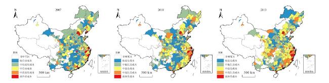
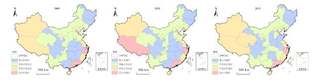
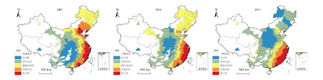
Urbanization is an important engine of economic growth. Urban housing condition, among others, is an important factor that may restrict the population migration from rural to urban areas. Using the Monitoring Survey Data of National Floating Population, Census data and other statistical data, this paper analyzes the spatial evolution of housing cost which is measured by the ratio of housing price to income and housing rent to income and empirically investigates its effect on the labor migration. According to spatial correlation index (Getis-Ord ), housing cost shows a strong trend of spatial autocorrelation, transformation between cold and hot areas of housing cost is closely related with spatial distribution of floating population. Then, Conditional Logit estimation results show that the increase of urban housing cost significantly leads to a decrease in the probability of migrant inflow, Which has larger inhibition effect for migrants who are poorly educated, younger and female laborers. This article proposes that loosening admittance for migrants on public rental housing and low-rent housing and increasing in urban public housing coverage may help the population agglomeration.
ZHANG Haifeng , ZHANG Jiazi , YAO Xianguo . Spatial Evolution of Housing Cost and Its Effect on Labor Migration in China[J]. Economic geography, 2019 , 39(7) : 31 -38 . DOI: 10.15957/j.cnki.jjdl.2019.07.005
表1 流动人口城市住房的获得途径/%Tab.1 Housing type of floating people in China/% |
| 现住房属性 | 全国样本 | 东部地区 | 中部地区 | 西部地区 |
|---|---|---|---|---|
| 租房 | 69.56 | 72.42 | 64.33 | 69.71 |
| 租住单位/雇主房 | 5.14 | 5.76 | 3.71 | 5.47 |
| 租住廉租房/公租房 | 0.40 | 0.23 | 0.30 | 0.80 |
| 租住私房 | 64.02 | 66.43 | 60.32 | 63.44 |
| 已购住房 | 17.21 | 11.95 | 24.80 | 18.91 |
| 已购商品房 | 13.60 | 10.74 | 19.81 | 12.50 |
| 已购政策性保障房 | 0.64 | 0.24 | 0.91 | 1.04 |
| 自建房 | 2.97 | 0.97 | 4.08 | 5.37 |
| 其他 | 13.23 | 15.63 | 15.86 | 11.38 |
| 样本数量 | 20 944 | 93 984 | 52 984 | 53 976 |
注:“其他”包括:单位/雇主提供免费房、租借房、就业场所、其他非正规居所等居住方式。 |
表2 城市特征变量说明Tab.2 Description of urban characteristic variables |
| 变量 | 观测值 | 均值 | 标准差 | 定义 |
|---|---|---|---|---|
| 房租—收入比 | 264 | 0.301 | 0.220 | 每月住房租金与各城市流动人口平均月收入的比值 |
| 房价—收入比 | 264 | 0.185 | 0.056 | 每平方住房价格与各城市城镇居民平均年收入的比值 |
| 人口密度 | 264 | 0.755 | 0.260 | 2013年城区人口(万人)/建成区面积(104×m2) |
| 医疗水平 | 264 | 1.999 | 1.440 | 2013年人均病床数、人均医生数和人均医院数的主成分分析得分值 |
| 教育水平 | 264 | 8.798 | 15.105 | 2013年全市普通高等学校数 |
| 失业率 | 264 | 0.049 | 0.039 | 2013年末城镇登记失业人员数/(登记失业人数+在岗职工人数) |
| 外省人口所占比例 | 264 | 0.048 | 0.086 | 2010年外省迁入人口/各市总人口 |
| 跨省迁移 | 264 | 0.435 | 0.495 | 户口所在地与流入地为不同省份 |
| 到北上广深的距离 | 264 | 639.570 | 403.150 | 某一城市到北上广深的最短地理距离(km) |
| 到高等级城市的距离 | 264 | 142.080 | 100.710 | 某一城市到高行政等级城市的最短地理距离(km) |
表3 劳动力个体特征变量Tab.3 Descriptive statistics of urban characteristic variables |
| 变量 | 观测值 | 均值 | 标准差 |
|---|---|---|---|
| 年龄 | 18 994 | 30.622 | 9.586 |
| 性别 | 18 994 | 0.596 | 0.490 |
| 受教育年限 | 18 994 | 9.921 | 2.845 |
| 婚姻状况(已婚=1) | 18 994 | 0.604 | 0.489 |
| 户籍(城镇=1) | 18 994 | 0.102 | 0.303 |
注:“2014年全国流动人口动态监测数据”询问了被调查者的受教育程度,本文将受教育程度转化受教育年限,对应关系如下:未上过学=0年,小学=6年,中学=9年,高中=12年,大学专科=15年,大学本科=16年,研究生=18年。 |
表4 住房成本的Moran's I检验Tab.4 Moran's I test of housing cost |
| 2007 | 2008 | 2009 | 2010 | 2011 | 2012 | 2013 | |
|---|---|---|---|---|---|---|---|
| 住房成本 | 0.158*** (9.732) | 0.185*** (11.39) | 0.214*** (13.22) | 0.245*** (15.08) | 0.263*** (16.16) | 0.271*** (16.62) | 0.243*** (14.93) |
注:***、**、*分别为99%、95%、90%下的显著性水平,括号内为Z值。 |
表5 住房成本对劳动力流向决策的影响:基本结果Tab.5 The overall impact of housing cost on labor force flowing |
| 解释变量 | 回归1 | 回归2 | 回归3 | 回归4 |
|---|---|---|---|---|
| 房租—收入比 | -1.961*** (0.065) | -1.510*** (0.078) | -1.019*** (0.077) | -1.267***(0.239) |
| 失业率 | - | -6.765*** (0.467) | -2.651*** (0.403) | -2.211** (1.109) |
| 人口密度 | - | 0.476*** (0.040) | -0.003 (0.041) | -0.306***(0.097) |
| 教育水平 | - | 0.547*** (0.011) | 0.473*** (0.015) | 0.742*** (0.042) |
| 医疗水平 | - | 0.127*** (0.009) | 0.136*** (0.010) | 0.021 (0.026) |
| 外省人口占比 | - | - | 3.903*** (0.113) | 3.863*** (0.225) |
| 是否跨省迁移 | - | - | 1.408*** (0.084) | 1.165*** (0.102) |
| 到北上广深的距离 | - | - | -0.0006*** (0.000) | 0.0029***(0.0002) |
| 到高级行政区的距离 | - | - | -0.0001 (0.000) | 0.00009 (0.0002) |
| 省固定效应 | 已控制 | 已控制 | 已控制 | 已控制 |
| 城市数量 | 264 | 264 | 264 | 67 |
| 个体数量 | 18 894 | 18 894 | 18 894 | 10 831 |
| 观测值 | 4 988 016 | 4 988 016 | 4 988 016 | 725 677 |
| LR chi2 | 18 222.60 | 28 319.47 | 30 262.80 | 10 041.61 |
| R2 | 0.0865 | 0.1344 | 0.1436 | 0.1052 |
注:***、**、*分别表示在1%、5%、10%上的显著性水平,括号内为标准差。 |
表6 不同地区住房成本对劳动力流向决策的影响Tab.6 The impact of housing cost on labor force flowing in different areas |
| 东部地区 | 中部地区 | 西部地区 | |
|---|---|---|---|
| 房租—收入比 | -2.717*** (0.147) | -0.268 (0.174) | -0.781*** (0.1605) |
| 其他城市特征变量 | 已控制 | 已控制 | 已控制 |
| 省固定效应 | 已控制 | 已控制 | 已控制 |
| 城市数量 | 89 | 102 | 73 |
| 个体数量 | 11 412 | 3 441 | 4 041 |
| 观测点数量 | 1 015 668 | 350 982 | 294 993 |
| LR chi2 | 15 792.94 | 3 768.54 | 5 565.04 |
| R2 | 0.1542 | 0.1184 | 0.1605 |
注:***、**、*分别表示在1%,5%,10%上的显著性水平;括号内为标准差;其他城市特征变量与表4的第(4)列回归一致。 |
表7 北上广住房成本上升对劳动力流入周边城市的影响Tab.7 The rising housing cost impact of Beijing, Shanghai, Guangzhou on labor force flowing of surrounding cities |
| 城市 | 区域内城市(%) | ||||
|---|---|---|---|---|---|
| 北京 | 京津冀 | 天津 (0.254) | 石家庄 (0.149) | 唐山 (0.023) | 秦皇岛 (0.044) |
| 上海 | 长三角 | 南京 (0.130) | 无锡 (0.06) | 杭州 (0.131) | 宁波 (0.087) |
| 广州 | 珠三角 | 深圳 (0.172) | 珠海 (0.041) | 东莞 (0.046) | 惠州 (0.040) |
表8 住房成本对劳动力流向决策的异质性影响Tab.8 The heterogeneous impact of housing cost on labor force flowing |
| 解释变量 | 全国 | 东部地区 | 中部地区 | 西部地区 |
|---|---|---|---|---|
| 房租—收入比 | -1.458***(0.216) | -3.526***(0.415) | -2.472***(0.591) | -0.377(0.389) |
| 高中*房租—收入比 | 1.006***(0.125) | 2.209***(0.245) | 0.302(0.329) | -1.157***(0.256) |
| 大专*房租—收入比 | 1.298***(0.174) | 3.862***(0.341) | -0.239(0.497) | -1.250***(0.369) |
| 本科及以上*房租—收入比 | 1.092***(0.250) | 4.185***(0.477) | -1.148(0.867) | -1.026**(0.518) |
| 1970—1980年出生*房租—收入比 | -0.526***(0.180) | -0.931***(0.356) | -0.312(0.502) | -0.389(0.336) |
| 1980—1990年出生*房租—收入比 | -0.503***(0.166) | -0.847***(0.328) | 0.143(0.468) | -0.073(0.304) |
| 1990年后出生*房租—收入比 | -1.174***(0.199) | -2.123***(0.382) | 0.749(0.548) | -0.028(0.363) |
| 婚姻(已婚=1)*房租—收入比 | 0.313**(0.132) | -0.452*(0.249) | 3.104***(0.370) | -0.397(0.244) |
| 性别(男性=1)*房租—收入比 | 0.435***(0.104) | 0.845***(0.194) | -0.246(0.277) | 0.289(0.197) |
| 户口(城镇=1)*房租—收入比 | 0.989***(0.149) | 1.029***(0.322) | 0.628(0.418) | 0.429(0.283) |
| 其他城市特征变量 | 已控制 | 已控制 | 已控制 | 已控制 |
| 省固定效应 | 已控制 | 已控制 | 已控制 | 已控制 |
| 城市数量 | 264 | 89 | 102 | 73 |
| 个体数量 | 18 894 | 11 412 | 3 441 | 4 041 |
| 观测值 | 4 988 016 | 1 015 668 | 350 982 | 294 993 |
| LR chi2 | 30 566.98 | 16 159.74 | 3 863.35 | 5 600.08 |
| R2 | 0.1451 | 0.1577 | 0.1214 | 0.1615 |
注:***、**、*分别表示在1%、5%、10%上的显著性水平;括号内为标准差。表9同。 |
表9 住房成本对劳动力流向决策的影响:稳健性分析Tab.9 Robustness test of housing cost on labor force flowing |
| 解释变量 | 回归1 | 回归2 | 回归3 | 回归4 |
|---|---|---|---|---|
| 房价—收入比 (2013) | -1.850*** (0.152) | - | - | - |
| 房价—收入比 (2012) | - | -0.988*** (0.154) | - | - |
| 房价—收入比 (2011—2013) | - | - | -1.541*** (0.147) | - |
| 房租—收入比 | - | - | - | -1.132*** (0.096) |
| 其他城市特征变量 | 已控制 | 已控制 | 已控制 | 已控制 |
| 省份固定效应 | 已控制 | 已控制 | 已控制 | 已控制 |
| 城市数量 | 264 | 264 | 264 | 264 |
| 个体数量 | 18 994 | 18 994 | 18 994 | 12 624 |
| 观测值 | 4 988 016 | 4 988 016 | 4 988 016 | 3 332 736 |
| LR chi2 | 30 216.68 | 30 104.50 | 30 175.71 | 21 110.47 |
| R2 | 0.1434 | 0.1429 | 0.1432 | 0.1500 |
| [1] |
|
| [2] |
|
| [3] |
周其仁. 逃得离的北上广,回不去的家乡[EB/OL]. 爱思想, http://www.aisixiang.com/data/105214.html, 2017-07-24.
|
| [4] |
彭国华. 技术能力匹配、劳动力流动与中国地区差距[J]. 经济研究, 2015(1):99-110.
|
| [5] |
陈心颖. 人口集聚对区域劳动生产率的异质性影响[J]. 人口研究, 2015(1):85-95.
|
| [6] |
蔡昉. 中国经济改革效应分析——劳动力重新配置的视角[J]. 经济研究, 2017(7):4-17.
|
| [7] |
|
| [8] |
|
| [9] |
|
| [10] |
|
| [11] |
高波, 陈健, 邹琳华. 区域房价差异、劳动力流动与产业升级[J]. 经济研究, 2012(1):66-79.
|
| [12] |
张莉, 何晶, 马润泓. 房价如何影响劳动力流动?[J]. 经济研究, 2017(8):155-170.
|
| [13] |
夏怡然, 陆铭. 城市间的“孟母三迁”[J]. 管理世界, 2015(10):78-90.
|
| [14] |
陆铭, 高虹, 佐藤宏. 城市规模与包容性就业[J]. 中国社会科学, 2012(10):47-66.
|
| [15] |
翟振武, 侯佳伟. 北京市外来人口聚居区——模式和发展趋势[J]. 人口研究, 2010(1):30-42.
|
| [16] |
|
| [17] |
|
/
| 〈 |
|
〉 |