
Spatial-Temporal Evolution and Regional Disparity of Economic High-Quality Development in the Yangtze River Economic Belt
Received date: 2019-05-27
Revised date: 2019-11-05
Online published: 2025-04-11
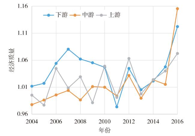
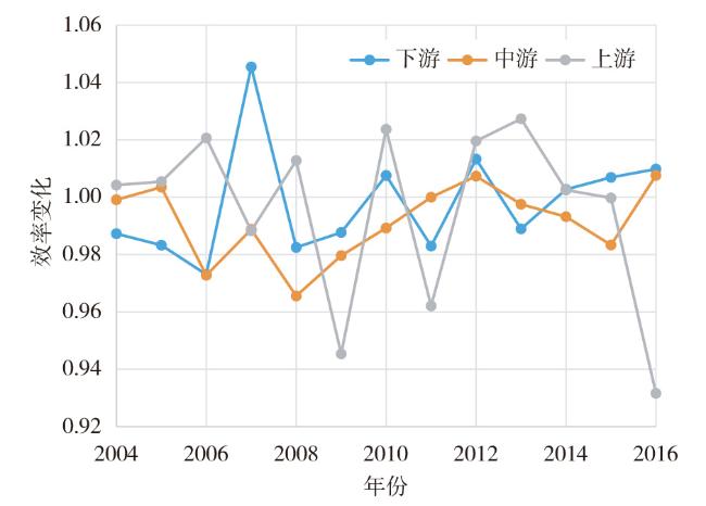
Achieving high-quality economic development under the background of the new era is the key to building a beautiful China. Based on the panel data of 108 cities in the Yangtze River Economic Belt from 2003 to 2016,the ML index and the Dagum Gini coefficient method were used to measure and analyze spatial-temporal evolution and regional disparity of economic quality,efficiency change and technological change. The results show that the economic quality,efficiency changes and technological changes are growing at an average annual rate of 2.48%,-0.53%,and 3.03%,technological progress is the driving force for the optimization of economic quality. The economic quality of the upper,middle and lower reaches shows periodic fluctuations over time,the average economic quality of the downstream is the highest,followed by the upstream and the lowest in the midstream. The spatial distribution pattern of high-value areas of economic quality has evolved from upper and lower areas to middle and lower reaches,the high-value area of efficiency change is a spatial agglomeration pattern of the middle reaches of the Yangtze River and the Yangtze River Delta urban agglomeration,high-value areas of technological change are distributed in the middle and upper reaches. The overall regional disparity in economic quality,efficiency change,and technological change has expanded,and the inter-regional gap is the main cause of the overall regional disparity.
WANG Xia , XU Xiaohong . Spatial-Temporal Evolution and Regional Disparity of Economic High-Quality Development in the Yangtze River Economic Belt[J]. Economic geography, 2020 , 40(3) : 5 -15 . DOI: 10.15957/j.cnki.jjdl.2020.03.002
表1 长江经济带108个城市Tab.1 108 cities in the Yangtze River Economic Belt |
| 省域 | 数量(个) | 城市 | ||
|---|---|---|---|---|
| 上海 | 1 | - | ||
| 江苏 | 13 | 南京、无锡、徐州、常州、苏州、南通、连云港、淮安、盐城、扬州、镇江、泰州、宿迁 | ||
| 浙江 | 11 | 杭州、宁波、温州、嘉兴、湖州、绍兴、金华、衢州、舟山、台州、丽水 | ||
| 安徽 | 16 | 合肥、芜湖、蚌埠、淮南、马鞍山、淮北、铜陵、安庆、黄山、滁州、阜阳、宿州、六安、亳州、池州、宣城 | ||
| 江西 | 11 | 南昌、景德镇、萍乡、九江、新余、鹰潭、赣州、吉安、宜春、抚州、上饶 | ||
| 湖北 | 12 | 武汉、黄石、十堰、宜昌、襄阳、鄂州、荆门、孝感、荆州、黄冈、咸宁、随州 | ||
| 湖南 | 13 | 长沙、株洲、湘潭、衡阳、邵阳、岳阳、常德、张家界、益阳、郴州、永州、怀化、娄底 | ||
| 重庆 | 1 | - | ||
| 四川 | 18 | 成都、自贡、攀枝花、泸州、德阳、绵阳、广元、遂宁、内江、乐山、南充、眉山、宜宾、广安、达州、雅安、巴中、资阳 | ||
| 贵州 | 4 | 贵阳、六盘水、遵义、安顺 | ||
| 云南 | 8 | 昆明、曲靖、玉溪、保山、昭通、丽江、普洱、临沧 | ||
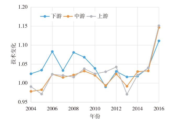
表2 长江经济带经济质量及增长源泉变化Tab.2 Economic quality and growth sources of the Yangtze River Economic Belt |
| 区域 | GTFP | MLEFFCH | MLTECH |
|---|---|---|---|
| 上游城市 | 1.0206 | 0.9952 | 1.0255 |
| 中游城市 | 1.0130 | 0.9913 | 1.0219 |
| 下游城市 | 1.0411 | 0.9976 | 1.0436 |
| 整体 | 1.0248 | 0.9947 | 1.0303 |
注:限于篇幅,未报告108个城市的具体结果。 |
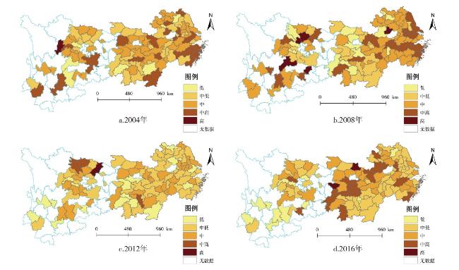
图7 经济质量空间分布格局演变趋势Fig.7 The evolution of the spatial distribution pattern of economic quality |
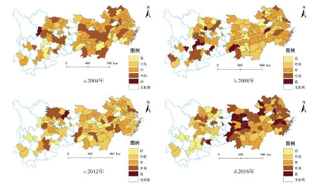
图8 效率变化空间分布格局演变趋势Fig.8 The evolution of spatial distribution pattern of efficiency change |
表3 经济质量的Dagum基尼系数及其来源Tab.3 Dagum Gini coefficient of economic quality and its source |
| 年份 | 总体区域差距 | 区域内差距 | 区域间差距 | 超变密度 | 贡献率(%) | ||
|---|---|---|---|---|---|---|---|
| 区域内差距 | 区域间差距 | 超变密度 | |||||
| 2004 | 0.0396 | 0.0137 | 0.0251 | 0.0008 | 34.60 | 63.38 | 2.02 |
| 2005 | 0.0377 | 0.0134 | 0.0212 | 0.0031 | 35.54 | 56.23 | 8.22 |
| 2006 | 0.0371 | 0.0123 | 0.0227 | 0.0021 | 33.15 | 61.19 | 5.66 |
| 2007 | 0.0413 | 0.0137 | 0.0235 | 0.0041 | 33.17 | 56.90 | 9.93 |
| 2008 | 0.0487 | 0.0167 | 0.0314 | 0.0006 | 34.29 | 64.48 | 1.23 |
| 2009 | 0.0430 | 0.0153 | 0.0229 | 0.0048 | 35.58 | 53.26 | 11.16 |
| 2010 | 0.0413 | 0.0147 | 0.0250 | 0.0016 | 35.59 | 60.53 | 3.87 |
| 2011 | 0.0757 | 0.0265 | 0.0453 | 0.0039 | 35.01 | 59.84 | 5.15 |
| 2012 | 0.0457 | 0.0150 | 0.0233 | 0.0074 | 32.82 | 50.98 | 16.19 |
| 2013 | 0.0393 | 0.0136 | 0.0244 | 0.0013 | 34.61 | 62.09 | 3.31 |
| 2014 | 0.0325 | 0.0116 | 0.0192 | 0.0017 | 35.69 | 59.08 | 5.23 |
| 2015 | 0.0346 | 0.0130 | 0.0209 | 0.0007 | 37.57 | 60.40 | 2.02 |
| 2016 | 0.0553 | 0.0200 | 0.0309 | 0.0044 | 36.17 | 55.88 | 7.96 |
表4 效率变化的Dagum基尼系数及其来源Tab.4 Dagum Gini coefficient of efficiency change and its source |
| 年份 | 总体区域差距 | 区域内差距 | 区域间差距 | 超变密度 | 贡献率(%) | ||
|---|---|---|---|---|---|---|---|
| 区域内差距 | 区域间差距 | 超变密度 | |||||
| 2004 | 0.0365 | 0.0131 | 0.0225 | 0.0009 | 35.89 | 61.64 | 2.47 |
| 2005 | 0.0340 | 0.0126 | 0.0198 | 0.0016 | 37.06 | 58.24 | 4.71 |
| 2006 | 0.0325 | 0.0109 | 0.0169 | 0.0047 | 33.54 | 52.00 | 14.46 |
| 2007 | 0.0339 | 0.0116 | 0.0190 | 0.0033 | 34.22 | 56.05 | 9.73 |
| 2008 | 0.0327 | 0.0114 | 0.0190 | 0.0023 | 34.86 | 58.10 | 7.03 |
| 2009 | 0.0381 | 0.0138 | 0.0213 | 0.0030 | 36.22 | 55.91 | 7.87 |
| 2010 | 0.0373 | 0.0136 | 0.0218 | 0.0019 | 36.46 | 58.45 | 5.09 |
| 2011 | 0.0623 | 0.0226 | 0.0383 | 0.0014 | 36.28 | 61.48 | 2.25 |
| 2012 | 0.0339 | 0.0119 | 0.0192 | 0.0028 | 35.10 | 56.64 | 8.26 |
| 2013 | 0.0365 | 0.0127 | 0.0212 | 0.0026 | 34.79 | 58.08 | 7.12 |
| 2014 | 0.0296 | 0.0102 | 0.0172 | 0.0022 | 34.46 | 58.11 | 7.43 |
| 2015 | 0.0295 | 0.0112 | 0.0179 | 0.0004 | 37.97 | 60.68 | 1.36 |
| 2016 | 0.0414 | 0.0134 | 0.0221 | 0.0059 | 32.37 | 53.38 | 14.25 |
表5 技术变化的Dagum基尼系数及其来源Tab.5 Dagum Gini coefficient of technical change and its source |
| 年份 | 总体区域差距 | 区域内差距 | 区域间差距 | 超变密度 | 贡献率(%) | ||
|---|---|---|---|---|---|---|---|
| 区域内差距 | 区域间差距 | 超变密度 | |||||
| 2004 | 0.0271 | 0.0090 | 0.0158 | 0.0023 | 33.21 | 58.30 | 8.49 |
| 2005 | 0.0283 | 0.0093 | 0.0132 | 0.0058 | 32.86 | 46.64 | 20.49 |
| 2006 | 0.0239 | 0.0072 | 0.0115 | 0.0052 | 30.13 | 48.12 | 21.76 |
| 2007 | 0.0214 | 0.0073 | 0.0137 | 0.0004 | 34.11 | 64.02 | 1.87 |
| 2008 | 0.0321 | 0.0104 | 0.0191 | 0.0026 | 32.40 | 59.50 | 8.10 |
| 2009 | 0.0196 | 0.0067 | 0.0108 | 0.0021 | 34.18 | 55.10 | 10.71 |
| 2010 | 0.0212 | 0.0076 | 0.0133 | 0.0003 | 35.85 | 62.74 | 1.42 |
| 2011 | 0.0403 | 0.0138 | 0.0220 | 0.0045 | 34.24 | 54.59 | 11.17 |
| 2012 | 0.0249 | 0.0085 | 0.0128 | 0.0036 | 34.14 | 51.41 | 14.46 |
| 2013 | 0.0280 | 0.0094 | 0.0141 | 0.0045 | 33.57 | 50.36 | 16.07 |
| 2014 | 0.0185 | 0.0066 | 0.0115 | 0.0004 | 35.68 | 62.16 | 2.16 |
| 2015 | 0.0179 | 0.0062 | 0.0115 | 0.0002 | 34.64 | 64.25 | 1.12 |
| 2016 | 0.0363 | 0.0135 | 0.0216 | 0.0012 | 37.19 | 59.50 | 3.31 |
| [1] |
高培勇, 杜创, 刘霞辉, 等. 高质量发展背景下的现代化经济体系建设:一个逻辑框架[J]. 经济研究, 2019(4):4-17.
|
| [2] |
任保平. 新时代中国经济从高速增长转向高质量发展:理论阐释与实践取向[J]. 学术月刊, 2018(3):66-74.
|
| [3] |
金碚. 关于“高质量发展”的经济学研究[J]. 中国工业经济, 2018(4):5-18.
|
| [4] |
任保平. 经济增长质量:经济增长理论框架的扩展[J]. 经济学动态, 2013(11):45-51.
|
| [5] |
魏敏, 李书昊. 新时代中国经济高质量发展水平的测度研究[J]. 数量经济技术经济研究, 2018(11):3-20.
|
| [6] |
唐毅南. 中国经济真是“粗放式增长”吗——中国经济增长质量的经验研究[J]. 学术月刊, 2014(12):82-96.
|
| [7] |
陈诗一, 陈登科. 雾霾污染、政府治理与经济高质量发展[J]. 经济研究, 2018(2):20-34.
|
| [8] |
|
| [9] |
李平, 付一夫, 张艳芳. 生产性服务业能成为中国经济高质量增长新动能吗[J]. 中国工业经济, 2017(12):5-21.
|
| [10] |
刘思明, 张世瑾, 朱惠东. 国家创新驱动力测度及其经济高质量发展效应研究[J]. 数量经济技术经济研究, 2019(4):3-23.
|
| [11] |
|
| [12] |
|
| [13] |
郝国彩, 徐银良, 张晓萌, 等. 长江经济带城市绿色经济绩效的溢出效应及其分解[J]. 中国人口·资源与环境, 2018(5):75-83.
|
| [14] |
邢贞成, 王济干, 张婕. 长江经济带全要素生态效率的时空分异与演变[J]. 长江流域资源与环境, 2018(4):792-799.
|
| [15] |
袁茜, 吴利华, 张平. 长江经济带一体化发展与高技术产业研发效率[J]. 数量经济技术经济研究, 2019(4):45-60.
|
| [16] |
|
| [17] |
|
| [18] |
易明, 李纲, 彭甲超, 等. 长江经济带绿色全要素生产率的时空分异特征研究[J]. 管理世界, 2018(11):178-179.
|
| [19] |
|
| [20] |
|
| [21] |
|
/
| 〈 |
|
〉 |
