
Spatial Econometric Analysis on the Influence of Elements Flow and Industrial Collaborative Agglomeration on Regional Economic Growth:Based on Manufacturing and Producer Services
Received date: 2020-05-23
Revised date: 2021-06-10
Online published: 2025-03-31
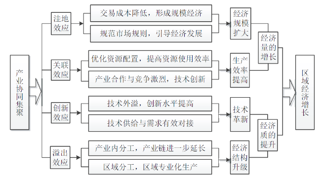
Taking manufacturing and producer services,which are closely related to industries,as an example,this paper studies the important role of industrial co-agglomeration in improving production efficiency and innovation ability,so as to realize the regional economy growth of "quantity" and "quality". Firstly,based on the industrial synergy agglomeration index,it measures the level of industrial co-agglomeration between manufacturing and producer services in 30 provinces of China from 2003 to 2016. Secondly,it explores the important role of industrial collaborative agglomeration on regional economic growth from the perspective of production efficiency and technological innovation by the means of the spatial measurement model. The results show: the industrial co-agglomeration can improve production efficiency,and promote innovation and economic growth,which has a significant space spillover effect and is of great significance to realize the regional economy growth of "quantity" and "quality". Moreover,the industrial co-agglomeration has a significant spatial spillover effect and has a positive guiding significance to the cross-regional cooperation of the economic development. Therefore,in the course of the current economic development,the regions should strengthen the integrated development consciousness,break through the regional boundary,strengthen the regional cooperation,and realize the common development on the basis of the regional advantages.
TANG Chang'an , QIU Jiawei , ZHANG Lijia , LI Hongyan . Spatial Econometric Analysis on the Influence of Elements Flow and Industrial Collaborative Agglomeration on Regional Economic Growth:Based on Manufacturing and Producer Services[J]. Economic geography, 2021 , 41(7) : 146 -154 . DOI: 10.15957/j.cnki.jjdl.2021.07.016
表1 变量的描述性统计Tab.1 Descriptive statistics of the variables |
| Variable | Obs | mean | Std. Dev. | Min | Max |
|---|---|---|---|---|---|
| LP | 510 | 10.863 | 0.723 | 8.338 | 12.409 |
| R | 510 | 2.661 | 0.106 | 1.858 | 2.533 |
| Hr | 510 | 9.856 | 1.048 | 6.752 | 11.937 |
| K | 510 | 5.398 | 0.888 | 3.326 | 7.746 |
| ED | 510 | 8.699 | 0.845 | 5.865 | 9.978 |
| Jt | 510 | 11.925 | 2.039 | 4.477 | 14.941 |
表2 空间面板模型的LM检验结果Tab.2 The LM test results of the space panel model |
| LM检验 | 地理矩阵(W1) | 经济地理矩阵(W2) | |||
|---|---|---|---|---|---|
| T值 | P值 | T值 | P值 | ||
| LM-lag | 57.886 | 0.000 | 100.262 | 0.000 | |
| LM-error | 78.724 | 0.000 | 109.881 | 0.000 | |
| R-lmlag | 48.366 | 0.000 | 87.792 | 0.000 | |
| R-lmerror | 73.201 | 0.000 | 88.945 | 0.000 | |
表3 空间计量模型回归结果Tab.3 Regression results of spatial econometric model |
| 变量 | 地理矩阵(W1) | 经济地理矩阵(W2) | |||||
|---|---|---|---|---|---|---|---|
| SLM(I)-re | SEM(I)-re | SDM(I)-re | SLM(I)-re | SEM(I)-re | SDM(I)-fe | ||
| c | 0.599(1.55) | 2.180***(3.72) | 1.729***(3.66) | 0.916***(2.43) | 2.201***(4.46) | - | |
| R | 0.490***(2.62) | 1.438***(4.83) | 1.123***(3.67) | 0.535***(2.87) | 1.262***(4.58) | 0.648**(1.98) | |
| Hr | 0.285***(7.83) | 0.569***(15.30) | 0.349***(7.60) | 0.340***(10.16) | 0.608***(24.33) | 0.411***(7.71) | |
| K | 0.057(1.37) | -0.0216(-0.52) | 0.057(1.35) | 0.041(0.98) | -0.027(-0.63) | 0.044*(1.04) | |
| ED | -0.0002**(-2.50) | -7.08e-06(-0.08) | -0.002*(-1.65) | -0.0001***(-1.58) | 0.00007***(0.843) | -5.0002***(-1.61) | |
| JT | 0.015(1.37) | 0.006***(0.54) | 0.007(0.62) | 0.009***(0.79) | 1.005(0.42) | 0.009(0.3996) | |
| W·R | - | - | -0.311(-0.90) | - | - | -0.269(-0.70) | |
| W·Hr | - | - | -0.099*(-1.66) | - | - | -0.092(-1.40) | |
| W·K | - | -0.181**(-2.52) | - | - | 0.257**(2.38) | ||
| W·ED | - | - | 0.0003***(2.23) | - | - | -0.0005**(-2.24) | |
| W·JT | - | 0.053**(2.50) | - | 0.088***(3.35) | |||
| ρ | 0.551***(10.33) | 0.6971***(9.93) | 0.454***(8.14) | 0.474***(9.73) | 0.501***(7.65) | 0.382***(5.72) | |
| R2 | 0.9179 | 0.9140 | 0.9230 | 0.9194 | 0.9153 | 0.9293 | |
| LogL | 142.5655 | 134.1495 | 241.4518 | 138.6455 | 123.3557 | 234.8033 | |
| SDM→SLM | 46.3953*** | - | - | 136.4427*** | |||
注:*、**、***表示在10%、5%、1%的显著水平,括号内为t值。表6同。 |
表4 变量的描述性统计Tab.4 Descriptive statistics of the variables |
| Variable | Obs | mean | Std. Dev. | Min | Max |
|---|---|---|---|---|---|
| CX | 510 | 12.158 | 17.401 | 0.230 | 104.993 |
| R | 510 | 2.655 | 0.339 | 1.411 | 3.531 |
| Hr | 510 | 2.180 | 0.105 | 1.858 | 2.543 |
| ZJ | 510 | 1.419 | 1.070 | 0.174 | 6.315 |
| Wg | 510 | 10.511 | 0.613 | 9.249 | 12.024 |
| Fdi | 510 | 11.973 | 2.036 | 4.477 | 14.941 |
| Inf | 510 | 9.947 | 0.887 | 6.426 | 11.714 |
表5 空间面板模型的LM检验结果Tab.5 The LM test results of the space panel model |
| LM检验 | 地理矩阵(W1) | 经济地理矩阵(W2) | |||
|---|---|---|---|---|---|
| T值 | P值 | T值 | P值 | ||
| LM-lag | 51.840 | 0.000 | 55.86 | 0.000 | |
| LM-error | 35.743 | 0.000 | 8.421 | 0.004 | |
| R-lmlag | 50.238 | 0.000 | 55.315 | 0.000 | |
| R-lmerror | 40.715 | 0.000 | 7.871 | 0.005 | |
表6 空间计量模型回归结果Tab.6 Regression results of spatial econometric model |
| 变量 | 地理矩阵(W1) | 经济地理矩阵(W2) | |||||
|---|---|---|---|---|---|---|---|
| SLM(I)-re | SEM(I)-fe | SDM(I)-re | SLM(I)-fe | SEM(I)-fe | SDM(I)-re | ||
| c | -10.177***(-10.92) | - | -4.722***(-5.57) | - | - | -1.357***(1.9030) | |
| R | 0.341***(5.69) | 0.280***(3.88) | 0.368***(5.56) | 0.209***(3.22 ) | 0.240***(3.43) | 0.1025***(0.1219) | |
| Hr | -0.192**(-2.55) | -0.283***(-3.76) | -0.226***(-2.97) | -0.206***(-2.85) | -0.202***(-2.71) | -0.016(0.0474) | |
| ZJ | -0.071(-1.13) | -0.125*(-1.87) | 0.086***(1.26) | -0.118*(-1.88) | -0.095(-1.41) | 0.333***(0.0474) | |
| Wg | 0.916***(9.88) | 1.392***(22.68) | 0.00001***(4.77) | 0.733***(7.36) | 1.408***(22.05) | 9.32e-061***(1.67e-06) | |
| Inf | 0.079***(4.41) | 0.067***(3.64) | 2.23e-06***(0.98) | 0.072***(4.06) | 0.079***(4.46) | 0.000103**(0.000017) | |
| FDI | -0.229***(-3.65) | -0.161**(-2.21) | -0.116***(6.16) | -0.241*(-3.46) | -0.228***(-3.32) | 0.0049(0.013) | |
| W·R | - | - | -0.114(0.450) | - | - | 1.338***(0.504) | |
| W·Hr | - | - | 0.100(1.01) | - | - | -0.223*(0.124) | |
| W·ZJ | - | - | 0.422***(4.43) | - | - | 0.164***(0.154) | |
| W·Wg | - | - | 0.00002***(2.50e-06) | - | - | -8.00e-07***(4.69e-06) | |
| W·Inf | - | - | 1.75e-06(0.42) | - | - | 0.000027***(0.000100) | |
| W·FDI | - | - | 0.025(0.76) | - | - | -0.1971***(0.0507) | |
| ρ | 0.271***(5.16) | - | 0.384***(7.55) | 0.459***(8.39) | - | 0.263***(0.139) | |
| R2 | 0.921 | 0.848 | 0.924 | 0.780 | 0.870 | 0.756 | |
| Log L | 121.156 | 121.156 | 127.595 | 231.288 | 137.853 | 108.631 | |
| SDM→SLM | - | - | 83.936*** | 76.929*** | |||
| [1] |
|
| [2] |
|
| [3] |
|
| [4] |
钟韵, 秦嫣然. 中国城市群的服务业协同集聚研究——基于长三角与珠三角的对比[J]. 广东社会科学, 2021(2):5-15,254.
|
| [5] |
刘书瀚, 于化龙. 生产性服务业集聚的经济增长效应研究——基于中国三大城市群的比较分析[J]. 中国科技论坛, 2020(6):44-53,145.
|
| [6] |
|
| [7] |
张明斗, 王亚男. 制造业、生产性服务业协同集聚与城市经济效率——基于“本地—邻地”效应的视角[J]. 山西财经大学学报, 2021, 43(6):5-28.
|
| [8] |
|
| [9] |
|
| [10] |
|
| [11] |
李骏, 刘洪伟, 陈银. 产业集聚、技术学习成本与区域经济增长——以中国省际高技术产业为例[J]. 软科学, 2018, 32(4):95-99.
|
| [12] |
汤长安, 张丽家. 产业协同集聚的区域技术创新效应研究——以制造业与生产性服务业为例[J]. 湖南师范大学社会科学学报, 2020, 49(3):140-148.
|
| [13] |
|
| [14] |
|
| [15] |
|
| [16] |
张军, 吴桂英, 张吉鹏. 中国省际物质资本存量估算:1952—2000[J]. 经济研究, 2004(10):35-44.
|
/
| 〈 |
|
〉 |